Let's say you want to find the average number of days for different employees to complete tasks. In addition, you want to calculate the average temperature for a specific day over a 10 year period of time. Calculating the average for a group of numbers can be done in several ways.
The AVERAGE function calculates the mean, which is the center of a set of numbers in a statistical distribution. There are three most common ways to determine the average:
Mean It is the arithmetic mean, which is calculated by adding a group of numbers and dividing them by the number of those numbers. For example, the average of the numbers 2, 3, 3, 5, 7, and 10 is 5, which is the result of dividing their sum of 30 by their number of 6.
Median The middle number of a group of numbers. Half of the numbers contain values \u200b\u200babove the median and half of the numbers contain values \u200b\u200bbelow the median. For example, the median for numbers 2, 3, 3, 5, 7, and 10 would be 4.
Fashion The most common number in a group of numbers. For example, the fashion for the numbers 2, 3, 3, 5, 7, and 10 would be 3.
With a symmetric distribution of the set of numbers, all three values \u200b\u200bof the central trend will coincide. In the rejected distribution of a group of numbers, they may be different.
Calculating the average of adjacent rows or columns
Follow the steps below.
Calculate the average outside of a continuous row or column
To accomplish this task, use the function AVERAGE ... Copy the table below onto a blank sheet.
Weighted average calculation
To accomplish this task, use the functions SUMPRODUCT and Sum ... In the VSIS example, the average prices paid per unit in three purchases are calculated, where each of them is intended for different units of goods on different units.
Copy the table below onto a blank sheet.
In most cases, the data is concentrated around some central point. Thus, to describe any data set, it is sufficient to indicate the average value. Let us consider sequentially three numerical characteristics that are used to estimate the mean value of the distribution: arithmetic mean, median and mode.
Average
The arithmetic mean (often called simply the mean) is the most common estimate of the mean of a distribution. It is the result of dividing the sum of all observed numerical values \u200b\u200bby their number. For a sample of numbers X 1, X 2, ..., X n, sample mean (denoted by ) is equal \u003d (X 1 + X 2 + ... + X n) / n, or
where is the sample mean, n - sample size, X i - i-th element of the sample.
Download a note in format or, examples in format
Consider the calculation of the arithmetic mean of the five-year average annual return of 15 very high-risk mutual funds (Figure 1).

Figure: 1. Average annual returns of 15 very high risk mutual funds
The sample mean is calculated as follows:

This is a good return, especially compared to 3-4% of the income that bank or credit union depositors received over the same period of time. If you order the returns, it is easy to see that eight funds have higher returns, and seven - below the average. The arithmetic mean acts as an equilibrium point so that low-income funds balance high-income funds. All elements of the sample are involved in calculating the average. None of the other estimates of the mean of the distribution has this property.
When to calculate the arithmetic mean.Since the arithmetic mean depends on all elements in the sample, the presence of extreme values \u200b\u200bsignificantly affects the result. In such situations, the arithmetic mean can distort the meaning of the numeric data. Therefore, when describing a dataset containing extreme values, it is necessary to indicate the median or arithmetic mean and median. For example, if you remove the RS Emerging Growth fund return from the sample, the sample average return of 14 funds will decrease by almost 1% to 5.19%.
Median
The median is the median of an ordered array of numbers. If the array does not contain duplicate numbers, then half of its elements will be less and half more than the median. If the sample contains extreme values, it is better to use the median rather than the arithmetic mean to estimate the mean. To calculate the median of a sample, you first need to order it.
This formula is ambiguous. Its result depends on whether the number is even or odd n:
- If the sample contains an odd number of elements, the median is (n + 1) / 2th element.
- If the sample contains an even number of elements, the median lies between the two mean elements of the sample and is equal to the arithmetic mean calculated over these two elements.
To compute the median of a sample of 15 very high-risk mutual funds, you first need to sort the data (Figure 2). Then the median will be opposite the number of the middle element of the sample; in our example # 8. Excel has a special function \u003d MEDIAN (), which works with unordered arrays too.

Figure: 2. Median 15 funds
So the median is 6.5. This means that the profitability of one half of the funds with a very high level of risk does not exceed 6.5, while the profitability of the other half does not exceed it. Note that the median of 6.5 is not much higher than the average of 6.08.
If we remove the return of the RS Emerging Growth fund from the sample, then the median of the remaining 14 funds will decrease to 6.2%, that is, not as significantly as the arithmetic mean (Fig. 3).

Figure: 3. Median 14 funds
Fashion
The term was first coined by Pearson in 1894. Fashion is the number that appears most often in the sample (most fashionable). Fashion describes well, for example, the typical reaction of drivers to a traffic signal to stop driving. A classic example of the use of fashion is choosing the size of a produced batch of shoes or a color for wallpaper. If a distribution has several modes, it is said to be multimodal or multimodal (has two or more "peaks"). The multimodality of the distribution provides important information about the nature of the variable under study. For example, in sociological surveys, if a variable represents a preference or attitude towards something, then multimodality can mean that there are several definitely different opinions. Multimodality also serves as an indicator that the sample is not homogeneous and the observations may be generated by two or more “overlaid” distributions. Unlike the arithmetic mean, outliers do not affect fashion. For continuously distributed random variables, for example, for indicators of average annual returns of mutual funds, the fashion sometimes does not exist at all (or does not make sense). Since these indicators can take on a wide variety of values, repeated values \u200b\u200bare extremely rare.
Quartiles
Quartiles are metrics that are most commonly used to estimate the distribution of data when describing the properties of large numeric samples. While the median splits the ordered array in half (50% of the array elements are less than the median and 50% more), quartiles split the ordered dataset into four parts. The Q 1, median, and Q 3 values \u200b\u200bare the 25th, 50th and 75th percentiles, respectively. The first quartile, Q 1, is the number that divides the sample into two parts: 25% of the items are less, and 75% are more than the first quartile.
The third quartile, Q 3, is the number that also divides the sample into two parts: 75% of the elements are less, and 25% is more than the third quartile.
To calculate quartiles in versions of Excel prior to 2007, the function \u003d QUARTILE (array; part) was used. Starting in Excel2010, two functions apply:
- \u003d QUARTILE.INC (array, part)
- \u003d QUARTILE.EXC (array, part)
These two functions give slightly different values \u200b\u200b(Figure 4). For example, when calculating quartiles of a sample containing data on the average annual return of 15 very high-risk mutual funds, Q 1 \u003d 1.8 or –0.7 for QUARTILE.INCL and QUARTILE.EXCL, respectively. By the way, the QUARTILE function used earlier corresponds to the modern QUARTILE function. To calculate quartiles in Excel using the above formulas, the data array does not need to be ordered.

Figure: 4. Calculation of quartiles in Excel
Let's emphasize again. Excel can calculate quartiles for one-dimensional discrete seriescontaining the values \u200b\u200bof a random variable. The calculation of quartiles for a frequency-based allocation is given in the section below.
Geometric mean
Unlike the arithmetic mean, the geometric mean allows you to estimate the degree of change in a variable over time. The geometric mean is the root n-th degree from the work n values \u200b\u200b(in Excel, the function \u003d SRGEOM is used):
G \u003d (X 1 * X 2 *… * X n) 1 / n
A similar parameter - the geometric mean of the rate of return - is determined by the formula:
G \u003d [(1 + R 1) * (1 + R 2) *… * (1 + R n)] 1 / n - 1,
where R i - rate of return for ith period of time.
For example, suppose that the initial investment is $ 100,000. By the end of the first year, it drops to $ 50,000, and by the end of the second year, it returns to the original $ 100,000. The rate of return on this investment over a two-year period equals 0, since the initial and final funds are equal to each other. However, the arithmetic average of the annual rates of return is \u003d (–0.5 + 1) / 2 \u003d 0.25 or 25%, since the rate of return in the first year R 1 \u003d (50,000 - 100,000) / 100,000 \u003d –0.5 , and in the second R 2 \u003d (100,000 - 50,000) / 50,000 \u003d 1. At the same time, the geometric mean of the profit rate for two years is: G \u003d [(1–0.5) * (1 + 1 )] 1/2 - 1 \u003d ½ - 1 \u003d 1 - 1 \u003d 0. Thus, the geometric mean more accurately reflects the change (more precisely, the absence of changes) in the volume of investments over a two-year period than the arithmetic mean.
Interesting Facts.First, the geometric mean will always be less than the arithmetic mean of the same numbers. Except when all the numbers taken are equal to each other. Secondly, considering the properties of a right-angled triangle, you can understand why the mean is called geometric. The height of a right-angled triangle, lowered to the hypotenuse, is the proportional average between the projections of the legs onto the hypotenuse, and each leg is the average proportional between the hypotenuse and its projection onto the hypotenuse (Fig. 5). This gives a geometric way of constructing the geometric mean of two (lengths) of segments: you need to build a circle on the sum of these two segments as in the diameter, then the height, restored from the point of their connection to the intersection with the circle, will give the desired value:

Figure: 5. Geometric nature of the geometric mean (drawing from Wikipedia)
The second important property of numerical data is their variationcharacterizing the degree of data variance. Two different samples can differ in both mean values \u200b\u200band variations. However, as shown in Fig. 6 and 7, the two samples may have the same variation but different means, or the same means and completely different variations. The data corresponding to polygon B in Fig. 7, changes much less than the data on which polygon A.

Figure: 6. Two symmetrical bell-shaped distributions with the same spread and different mean values

Figure: 7. Two symmetrical bell-shaped distributions with the same mean values \u200b\u200band different scatter
There are five estimates of data variation:
- scope,
- interquartile range,
- dispersion,
- standard deviation,
- the coefficient of variation.
Scope
The range is the difference between the largest and smallest elements of the sample:
Swipe \u003d X Max - X Min
The range of a sample containing data on the average annual returns of 15 very high-risk mutual funds can be calculated using an ordered array (see Figure 4): Span \u003d 18.5 - (–6.1) \u003d 24.6. This means that the difference between the highest and the lowest average annual return of funds with a very high level of risk is 24.6%.
Span measures the overall spread of the data. While sample size is a very simple estimate of the overall spread of the data, its weakness is that it does not take into account exactly how the data is distributed between the minimum and maximum elements. This effect is clearly seen in Fig. 8, which illustrates samples having the same span. Scale B demonstrates that if the sample contains at least one extreme value, the sample span is a very imprecise estimate of the dispersion of the data.

Figure: 8. Comparison of three samples with the same range; the triangle symbolizes the support of the balance and its location corresponds to the mean of the sample
Interquartile range
The interquartile, or mean, range is the difference between the third and first quartiles of the sample:
Interquartile range \u003d Q 3 - Q 1
This value makes it possible to estimate the spread of 50% of the elements and ignore the influence of extreme elements. The interquartile range of a sample containing data on the average annual return of 15 very high risk mutual funds can be calculated using the data in Fig. 4 (for example, for the QUARTILE.EXC function): Interquartile range \u003d 9.8 - (–0.7) \u003d 10.5. The interval bounded by the numbers 9.8 and –0.7 is often called the middle half.
It should be noted that the values \u200b\u200bof Q 1 and Q 3, and hence the interquartile range, do not depend on the presence of outliers, since their calculation does not take into account any value that would be less than Q 1 or more than Q 3. The sum of quantitative characteristics such as the median, the first and third quartiles, and the interquartile range, which are not affected by outliers, are called robust measures.
While the range and interquartile range provide an estimate of the overall and mean spread of the sample, respectively, none of these estimates take into account how the data are distributed. Dispersion and standard deviationare devoid of this disadvantage. These indicators allow you to assess the degree of fluctuation of data around the average. Sample variance is an approximation of the arithmetic mean, calculated from the squares of the differences between each sample element and the sample mean. For a sample X 1, X 2, ... X n, the sample variance (denoted by the symbol S 2 is given by the following formula:

In general, the sample variance is the sum of the squares of the differences between the elements of the sample and the sample mean, divided by the value equal to the sample size minus one:

where - arithmetic mean, n - sample size, X i - ith sample element X... In Excel before 2007, the \u003d VARP () function was used to calculate the sample variance; since 2010, the \u003d VARV () function is used.
The most practical and widely accepted estimate of the spread of the data is standard sample deviation... This indicator is denoted by the symbol S and is equal to the square root of the sample variance:

In Excel prior to 2007, the \u003d STDEV () function was used to calculate the standard sample deviation; since 2010, the \u003d STDEV.V () function is used. For the calculation of these functions, the dataset may be unordered.
Neither sample variance nor standard sample deviation can be negative. The only situation in which indicators S 2 and S can be zero is if all elements of the sample are equal to each other. In this highly improbable case, the span and interquartile range are also zero.
Numerical data is inherently volatile. Any variable can take on many different values. For example, different mutual funds have different rates of return and loss. Due to the variability of numerical data, it is very important to study not only the estimates of the mean, which are cumulative in nature, but also the estimates of variance, which characterize the dispersion of the data.
Variance and standard deviation allow you to estimate the spread of data around the mean, in other words, to determine how many sample elements are less than the mean, and how many are more. Dispersion has some valuable mathematical properties. However, its value is the square of the unit of measure - square percentage, square dollar, square inch, etc. Therefore, the natural measure of variance is the standard deviation, which is expressed in common units of measure - percent of income, dollars, or inches.
The standard deviation allows you to estimate the amount of fluctuation of the sample elements around the mean. In almost all situations, the majority of the observed values \u200b\u200blie in the interval plus or minus one standard deviation from the mean. Therefore, knowing the arithmetic mean of the sample elements and the standard sample deviation, it is possible to determine the interval to which the bulk of the data belongs.
The standard deviation of the return on the 15 very high-risk mutual funds is 6.6 (Figure 9). This means that the profitability of the bulk of funds differs from the average value by no more than 6.6% (i.e. fluctuates in the range from - S \u003d 6.2 - 6.6 \u003d -0.4 to + S \u003d 12.8). In fact, in this interval lies the five-year average annual return of 53.3% (8 out of 15) funds.

Figure: 9. Standard sample deviation
Note that as the squared differences are added, the sample farther from the mean gains more weight than the closer sample. This property is the main reason that the arithmetic mean is most often used to estimate the mean of a distribution.
The coefficient of variation
Unlike previous estimates of the spread, the coefficient of variation is a relative estimate. It is always measured as a percentage, not the unit of the original data. The coefficient of variation, denoted by CV, measures the dispersion of the data relative to the mean. The coefficient of variation is equal to the standard deviation divided by the arithmetic mean and multiplied by 100%:

where S - standard sample deviation, - sample mean.
The coefficient of variation allows you to compare two samples, the elements of which are expressed in different units of measurement. For example, a mail delivery manager intends to renew the truck fleet. When loading packages, there are two types of restrictions to consider: weight (in lbs) and volume (in cubic feet) of each package. For a sample of 200 bags, suppose the average weight is 26.0 pounds, the standard deviation of weight is 3.9 pounds, the average bag volume is 8.8 cubic feet, and the standard deviation is 2.2 cubic feet. How do you compare the weight and volume spread of bags?
Since the units of measure for weight and volume differ from each other, the manager must compare the relative spread of these values. The coefficient of variation of weight is CV W \u003d 3.9 / 26.0 * 100% \u003d 15%, and the coefficient of variation of volume CV V \u003d 2.2 / 8.8 * 100% \u003d 25%. Thus, the relative spread in packet volume is much larger than the relative spread in their weight.
Distribution form
The third important property of the sample is the shape of its distribution. This distribution can be symmetrical or asymmetric. To describe the shape of the distribution, it is necessary to calculate its mean and median. If these two indicators coincide, the variable is considered symmetrically distributed. If the mean value of a variable is greater than the median, its distribution has a positive skewness (Fig. 10). If the median is greater than the mean, the distribution of the variable is negatively skewed. Positive skewness occurs when the mean increases to unusually high values. Negative skewness occurs when the mean decreases to unusually small values. A variable is symmetrically distributed if it does not take any extreme values \u200b\u200bin either direction, so that the high and low values \u200b\u200bof the variable balance each other.

Figure: 10. Three types of distributions
The data shown on the A-scale have negative skewness. This figure shows a long tail and a skew to the left caused by unusually low values. These extremely small values \u200b\u200bshift the average to the left, and it becomes less than the median. The data shown on the B scale are symmetrically distributed. The left and right halves of the distribution are their mirror images. Large and small values \u200b\u200bcancel each other out, and mean and median are equal. The data shown on the B scale are positively skewed. This figure shows a long tail and a skew to the right caused by unusually high values. These too high values \u200b\u200bshift the average to the right, and it becomes larger than the median.
In Excel, descriptive statistics can be obtained using the add-in Analysis package... Go through the menu Data → Data analysis, in the window that opens, select the line Descriptive statistics and click Ok... In the window Descriptive statistics be sure to indicate Input interval(fig. 11). If you want to see descriptive statistics on the same sheet as the original data, select the radio button Output interval and specify the cell where you want to place the upper left corner of the output statistics (in our example, $ C $ 1). If you want to output data to a new sheet or to a new workbook, simply select the appropriate radio button. Check the box next to Summary statistics... Optionally, you can also choose Difficulty level,kth smallest andkth largest.
If on deposit Data in the area of Analysis you do not have an icon displayed Data analysis, you must first install the add-on Analysis package (see, for example).

Figure: 11. Descriptive statistics of the five-year average annual return of funds with very high levels of risk, calculated using the add-in Data analysisexcel programs
Excel calculates a variety of statistics discussed above: mean, median, mode, standard deviation, variance, range ( interval), minimum, maximum and sample size ( score). In addition, Excel calculates some statistics that are new to us: standard error, kurtosis, and skewness. Standard error equal to the standard deviation divided by the square root of the sample size. Asymmetry characterizes the deviation from the symmetry of the distribution and is a function that depends on the cube of differences between the sample elements and the mean. Kurtosis is a measure of the relative concentration of data around the mean versus the tails of the distribution and is dependent on the differences between the sample and the mean raised to the fourth power.
Computing descriptive statistics for a population
The mean, spread, and shape of the distribution discussed above are characteristics determined from the sample. However, if the dataset contains numeric dimensions for the entire population, you can calculate its parameters. These parameters include the mathematical expectation, variance and standard deviation of the general population.
Expected value is equal to the sum of all values \u200b\u200bof the general population divided by the size of the general population:

where µ - expected value, X i- i-th observation of a variable X, N - the volume of the general population. Excel uses the same function to calculate the mathematical expectation as for the arithmetic mean: \u003d AVERAGE ().
Population variance equal to the sum of the squares of the differences between the elements of the general population and mat. expectation divided by the size of the general population:

where σ 2 - variance of the general population. In Excel prior to 2007, the \u003d VARP () function is used to calculate the variance of the population, since 2010 \u003d VARP.G ().
Population standard deviation equals the square root of the population variance:

In Excel prior to 2007, the \u003d STDEVP () function is used to calculate the population standard deviation, since 2010 \u003d STDEV.Y (). Note that the formulas for population variance and standard deviation are different from the formulas for sample variance and standard deviation. When calculating sample statistics S 2 and S the denominator of the fraction is n - 1, and when calculating the parameters σ 2 and σ - the volume of the general population N.
Rule of thumb
In most situations, a large proportion of observations are concentrated around the median, forming a cluster. In datasets with positive skewness, this cluster is located to the left (i.e., below) the mathematical expectation, and in datasets with negative skewness, this cluster is located to the right (i.e., above) the mathematical expectation. For symmetric data, the mean and median are the same, and observations are concentrated around the mean, forming a bell-shaped distribution. If the distribution does not have a pronounced skewness, and the data is concentrated around a certain center of gravity, a rule of thumb can be applied to assess the variability, which says: if the data have a bell-shaped distribution, then approximately 68% of observations are no more than one standard deviation from the mathematical expectation. approximately 95% of observations are no more than two standard deviations from the mathematical expectation, and 99.7% of observations are no more than three standard deviations from the mathematical expectation.
Thus, the standard deviation, which is an estimate of the mean variation around the mean, helps to understand how observations are distributed and to identify outliers. It follows from a rule of thumb that for bell-shaped distributions, only one value in twenty differs from the mathematical expectation by more than two standard deviations. Therefore, values \u200b\u200boutside the interval µ ± 2σcan be considered outliers. Moreover, only three out of 1000 observations differ from the mathematical expectation by more than three standard deviations. Thus, values \u200b\u200boutside the interval µ ± 3σ are almost always outliers. For distributions that are highly skewed or not bell-shaped, the Biename-Chebyshev empirical rule can be applied.
More than a hundred years ago mathematicians Biename and Chebyshev independently discovered the useful property of the standard deviation. They found that for any dataset, regardless of the shape of the distribution, the percentage of observations lying at a distance not exceeding k standard deviations from mathematical expectation, not less (1 – 1/ k 2) * 100%.
For example, if k \u003d 2, the Biename-Chebyshev rule states that at least (1 - (1/2) 2) x 100% \u003d 75% of observations must lie in the interval µ ± 2σ... This rule is true for anyone kgreater than one. The Biename-Chebyshev rule is very general and is valid for any kind of distribution. It indicates the minimum number of observations, the distance from which to the mathematical expectation does not exceed a given value. However, if the distribution is bell-shaped, the rule of thumb is more accurate in estimating the concentration of data around the expected value.
Computing descriptive statistics for a frequency-based distribution
If the original data is not available, the frequency distribution becomes the only source of information. In such situations, you can calculate approximate values \u200b\u200bof quantitative distribution indicators, such as arithmetic mean, standard deviation, quartiles.
If the sample data is presented in the form of a frequency distribution, an approximate value of the arithmetic mean can be calculated, assuming that all values \u200b\u200bwithin each class are concentrated at the midpoint of the class:

where - sample mean, n - number of observations, or sample size, from - the number of classes in the frequency distribution, m j - midpoint j-go class, f j is the frequency corresponding j-th class.
To calculate the standard deviation from the frequency distribution, it is also assumed that all values \u200b\u200bwithin each class are centered at the midpoint of the class.

To understand how the quartiles of the series are determined based on frequencies, let us consider the calculation of the lower quartile based on data for 2013 on the distribution of the population of Russia by average per capita money income (Fig. 12).

Figure: 12. The share of the population of Russia with average per capita money incomes on average per month, rubles
To calculate the first quartile of an interval variation series, you can use the formula:

where Q1 is the value of the first quartile, хQ1 is the lower limit of the interval containing the first quartile (the interval is determined by the cumulative frequency, the first exceeding 25%); i is the size of the interval; Σf is the sum of the frequencies of the entire sample; probably always equal to 100%; SQ1-1 is the cumulative frequency of the interval preceding the interval containing the lower quartile; fQ1 is the frequency of the interval containing the lower quartile. The formula for the third quartile differs in that in all places Q3 should be used instead of Q1, and ¾ should be substituted for ¼.
In our example (Fig. 12), the lower quartile is in the range 7000.1 - 10,000, the cumulative frequency of which is 26.4%. The lower limit of this interval is 7000 rubles, the value of the interval is 3000 rubles, the cumulative frequency of the interval preceding the interval containing the lower quartile is 13.4%, the frequency of the interval containing the lower quartile is 13.0%. Thus: Q1 \u003d 7000 + 3000 * (¼ * 100 - 13.4) / 13 \u003d 9677 rubles.
Pitfalls with descriptive statistics
In this post, we looked at how to describe a dataset using various statistics that estimate its mean, spread, and distribution. The next step is data analysis and interpretation. Until now, we have studied the objective properties of data, and now we turn to their subjective interpretation. Two mistakes lie in wait for the researcher: an incorrectly chosen subject of analysis and an incorrect interpretation of the results.
The analysis of the performance of 15 very high risk mutual funds is quite impartial. It led to completely objective conclusions: all mutual funds have different returns, the spread of fund returns ranges from –6.1 to 18.5, and the average return is 6.08. The objectivity of data analysis is ensured by the correct choice of total quantitative distribution indicators. Several methods of estimating the mean and spread of the data were considered, their advantages and disadvantages were indicated. How do you choose the right statistics to provide objective and unbiased analysis? If the distribution of your data is slightly skewed, should you choose the median over the arithmetic mean? Which indicator more accurately characterizes the spread of the data: standard deviation or range? Should one point to a positive distribution skew?
On the other hand, data interpretation is a subjective process. Different people come to different conclusions when they interpret the same results. Everyone has their own point of view. Someone considers the total indicators of the average annual return of 15 funds with a very high level of risk to be good and is quite satisfied with the income received. Others may think that these funds have too low a return. Thus, subjectivity should be compensated for by honesty, neutrality and clarity of conclusions.
Ethical issues
Data analysis is inextricably linked to ethical issues. One should be critical of the information disseminated by newspapers, radio, television and the Internet. Over time, you will learn to be skeptical not only about the results, but also about the goals, subject matter and objectivity of the research. The famous British politician Benjamin Disraeli said it best of all: "There are three types of lies: lies, blatant lies and statistics."
As noted in the note, ethical issues arise in the selection of results to be reported. Both positive and negative results should be published. In addition, when making a report or a written report, the results must be presented in an honest, neutral and objective manner. Distinguish between unsuccessful and dishonest presentation. To do this, it is necessary to determine what the speaker's intentions were. Sometimes the presenter ignores important information, and sometimes it deliberately (for example, if he uses the arithmetic mean to estimate the average value of obviously asymmetric data in order to get the desired result). It is also unfair to gloss over results that do not correspond to the point of view of the researcher.
Used materials from the book Levin and other Statistics for managers. - M .: Williams, 2004 .-- p. 178-209
QUARTILE function is retained for compatibility with earlier versions of Excel
Arithmetic mean is a statistical indicator that demonstrates the average value of a given data array. Such an indicator is calculated as a fraction, the numerator of which is the sum of all the values \u200b\u200bof the array, and the denominator is their number. The arithmetic mean is an important coefficient that is used in household calculations.
The meaning of the coefficient
Arithmetic mean is an elementary indicator for comparing data and calculating an acceptable value. For example, different stores sell a can of beer from a specific manufacturer. But in one store it costs 67 rubles, in another - 70 rubles, in the third - 65 rubles, and in the last - 62 rubles. Quite a large spread of prices, so the buyer will be interested in the average cost of the can, so that when buying a product, he can compare his costs. On average, a can of beer in the city has a price:
Average price \u003d (67 + 70 + 65 + 62) / 4 \u003d 66 rubles.
Knowing the average price, it is easy to determine where it is profitable to buy a product, and where you will have to overpay.
The arithmetic mean is constantly used in statistical calculations in cases where a homogeneous data set is analyzed. In the example above, this is the price of a can of one brand of beer. However, we cannot compare the price of beer from different manufacturers or the price of beer and lemonade, since in this case the range of values \u200b\u200bwill be greater, the average price will be blurred and unreliable, and the very meaning of the calculations will be distorted to the cartoonish “average temperature in a hospital”. To calculate heterogeneous data sets, the arithmetic weighted average is used, when each value is weighted.
Calculating the arithmetic mean
The calculation formula is extremely simple:
P \u003d (a1 + a2 + ... an) / n,
where an is the value of the quantity, n is the total number of values.
What can this indicator be used for? The first and most obvious application is statistics. Almost every statistical study uses an arithmetic mean. This can be the average age at marriage in Russia, the average grade in a subject for a student, or the average spending on food per day. As discussed above, without considering weights, calculating averages can produce strange or absurd values.
For example, the President of the Russian Federation made a statement that according to statistics, the average salary of a Russian is 27,000 rubles. For most people in Russia, this level of wages seemed absurd. It is not surprising if, when calculating, we take into account the income of oligarchs, heads of industrial enterprises, large bankers on the one hand, and the salaries of teachers, cleaners and salesmen on the other. Even the average salaries in one specialty, for example, an accountant, will have significant differences in Moscow, Kostroma and Yekaterinburg.
How to calculate averages for dissimilar data
In payroll situations, it is important to consider the weight of each value. This means that the salaries of oligarchs and bankers would receive a weight of, for example, 0.00001, and the salaries of salesmen - 0.12. These are figures from the ceiling, but they roughly illustrate the prevalence of oligarchs and sellers in Russian society.
Thus, to calculate the average or average value in a heterogeneous data set, it is required to use the arithmetic weighted average. Otherwise, you will receive an average salary in Russia at the level of 27,000 rubles. If you want to know your average score in mathematics or the average number of goals scored by the selected hockey player, then the arithmetic mean calculator is for you.
Our program is a simple and convenient calculator for calculating the arithmetic mean. To perform calculations, you only need to enter the parameter values.
Let's look at a couple of examples
Average score calculation
Many teachers use the arithmetic mean method to determine the annual grade for a subject. Let's say a child gets the following math quarter marks: 3, 3, 5, 4. What annual grade will the teacher give him? Let's use a calculator and calculate the arithmetic mean. First, select the appropriate number of fields and enter the score values \u200b\u200bin the cells that appear:
(3 + 3 + 5 + 4) / 4 = 3,75
The teacher will round the value in favor of the student, and the student will receive a solid four in a year.
Calculation of candies eaten
Let's illustrate some of the absurdity of the arithmetic mean. Let's imagine that Masha and Vova had 10 candies. Masha ate 8 candies, and Vova - only 2. How many candies did each child eat on average? With the help of a calculator, it is easy to calculate that, on average, children ate 5 candies, which is completely contrary to reality and common sense. This example shows that the arithmetic mean is important to calculate for meaningful datasets.
Conclusion
The calculation of the arithmetic mean is widely used in many scientific fields. This indicator is popular not only in statistical calculations, but also in physics, mechanics, economics, medicine or finance. Use our calculators as an assistant for solving arithmetic mean problems.
Average salary ... Average life expectancy ... Almost every day we hear these phrases used to describe a set of one single number. But oddly enough, "average value" is a rather insidious concept, often misleading an ordinary person inexperienced in mathematical statistics.
What is the problem?
The average value most often means the arithmetic mean, which varies greatly under the influence of isolated facts or events. And you won't get a real idea of \u200b\u200bhow exactly the values \u200b\u200bthat you are studying are distributed.
Let's take a classic example with an average salary.
Some abstract company has ten employees. Nine of them receive a salary of about 50,000 rubles, and one of them is 1,500,000 rubles (by a strange coincidence, he is also the general director of this company).
The average value in this case will be 195,150 rubles, which you must agree is wrong.
What methods of calculating the average are there?
The first way is to calculate the already mentioned arithmetic mean, which is the sum of all values \u200b\u200bdivided by their number.

- x - arithmetic mean;
- x n - specific meaning;
- n - number of values.
- Works well with a normal distribution of sample values;
- Easy to calculate;
- Intuitively understandable.
- Doesn't give a real idea of \u200b\u200bthe distribution of values;
- An unstable quantity that is easily emitted (as is the case with the CEO).
The second way is to calculate fashion, that is, the most common value.

- M 0 - fashion;
- x 0 - the lower boundary of the interval that contains the fashion;
- n is the size of the interval;
- f m - frequency (how many times in a row this or that value occurs);
- f m-1 - frequency of the interval preceding the modal;
- f m + 1 - frequency of the interval following the modal.
- Great for getting an idea of \u200b\u200bpublic opinion;
- Good for non-numeric data (season colors, bestsellers, ratings);
- Easy to understand.
- Fashion may simply not be (no repetitions);
- There can be several mods (multimodal distribution).
The third way is to calculate medians, that is, the value that divides the ordered sample into two halves and is between them. And if there is no such value, then the arithmetic mean between the boundaries of the halves of the sample is taken as the median.

- M e - median;
- x 0 - the lower boundary of the interval that contains the median;
- h is the size of the interval;
- f i - frequency (how many times in a row this or that value occurs);
- S m-1 - the sum of the frequencies of the intervals preceding the median;
- f m is the number of values \u200b\u200bin the median interval (its frequency).
- Gives the most realistic and representative assessment;
- Resistant to emissions.
- It is more difficult to compute, since the sample must be ordered before computation.
We have covered the main methods for finding the average, called measures of the central trend(in fact, there are more of them, but these are the most popular).
Now let's go back to our example and calculate all three variants of the average using special Excel functions:
- AVERAGE (number1; [number2]; ...) - a function for determining the arithmetic mean;
- FASHION.ONE (number1; [number2]; ...) - fashion function (in older versions of Excel, MODA (number1; [number2]; ...));
- MEDIAN (number1; [number2]; ...) - a function for finding the median.
And here are the values \u200b\u200bwe got:
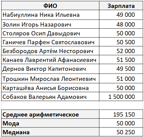
In this case, fashion and median characterize the average salary in a company much better.
But what to do when the sample contains not 10 values, as in the example, but millions? In Excel, this cannot be calculated, but in the database where your data is stored, no problem.
Calculating the arithmetic mean in SQL
Everything is quite simple here, since SQL provides a special AVG aggregate function.
And to use it, it is enough to write the following query:
Computing SQL fashion
SQL does not have a separate function for finding the mod, but it can be easily and quickly written by yourself. To do this, we need to find out which of the salaries is most often repeated and choose the most popular.
Let's write a request:
/ * WITH TIES must be added to TOP () if the set is multimodal, that is, the set has several mods * / SELECT TOP (1) WITH TIES salary AS "Salary mode" FROM employees GROUP BY salary ORDER BY COUNT (*) DESC
Calculating the median in SQL
As with fashion, SQL does not have a built-in function for calculating the median, but there is a universal function for calculating PERCENTILE_CONT percentiles.
It all looks like this:
/ * In this case, the percentile is 0.5 and will be the median * / SELECT TOP (1) PERCENTILE_CONT (0.5) WITHIN GROUP (ORDER BY salary) OVER () AS "Median salary" FROM employees
It is better to read more about how the PERCENTILE_CONT function works in the Microsoft and Google BigQuery help.
What method should you use?
From the above, it follows that the median is the best way to calculate the average.
But it's not always the case. If you are working with an average, then beware of multimodal distribution:
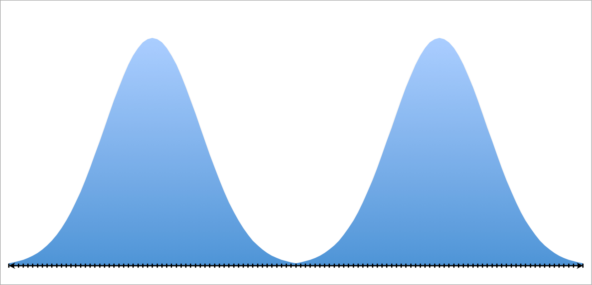
The graph shows a bimodal distribution with two peaks. Such a situation may arise, for example, when voting in elections.
In this case, the arithmetic mean and median are values \u200b\u200bthat are somewhere in between and they will not say anything about what is really happening and it is better to immediately recognize that you are dealing with a bimodal distribution by reporting two modes.
Better yet, divide the sample into two groups and collect statistics for each.
Output:
When choosing a method for finding the average, it is necessary to take into account the presence of outliers, as well as the normal distribution of values \u200b\u200bin the sample.
The final choice of the measure of the central trend always lies with the analyst.
Remember!
To find arithmetic mean, you need to add all the numbers and divide their sum by their number.
Find the arithmetic mean of 2, 3, and 4.
Let's denote the arithmetic mean by the letter "m". By the definition above, we find the sum of all numbers.
Divide the resulting amount by the number of numbers taken. We have three numbers by condition.
As a result, we get arithmetic mean formula:

What is the arithmetic mean for?
In addition to the fact that it is constantly suggested to be found in the lessons, finding the arithmetic mean is very useful in life.
For example, let's say you decide to sell soccer balls. But since you are new to this business, it is completely incomprehensible at what price to sell balls to you.
Then you decide to find out at what price competitors are already selling soccer balls in your area. Let's find out the prices in stores and draw up a table.
The prices for balls in stores were completely different. What price should we choose for selling a soccer ball?
If you choose the lowest one (290 rubles), then we will sell the goods at a loss. If you choose the highest one (360 rubles), then buyers will not buy soccer balls from us.
We need an average price. Here comes to the rescue average.
Let's calculate the arithmetic mean of the prices for soccer balls:
average price =
=
290 + 360 + 310
3
= 320
rub.960
3
Thus, we got an average price (320 rubles), at which we can sell a soccer ball not too cheaply and not too expensive.
Average travel speed
Closely related to the arithmetic mean is the concept average speed.
Observing the movement of transport in the city, you can see that cars are accelerating and going at high speed, then slowing down and going at low speed.
There are many such sections along the route of vehicles. Therefore, for the convenience of calculations, the concept of the average speed of movement is used.
Remember!
The average speed of movement is the entire distance traveled divided by the entire time of movement.

Consider a medium speed problem.
Problem number 1503 from the textbook "Vilenkin grade 5"
The car moved for 3.2 hours on the highway at a speed of 90 km / h, then 1.5 hours on a dirt road at a speed of 45 km / h, and finally 0.3 hours on a country road at a speed of 30 km / h. Find the average speed of the car along the way.
To calculate the average speed of movement, you need to know the entire path traveled by the car, and all the time that the car was moving.
S 1 \u003d V 1 t 1S 1 \u003d 90 3.2 \u003d 288 (km)
- highway.S 2 \u003d V 2 t 2
S 2 \u003d 45 1.5 \u003d 67.5 (km) - dirt road.
S 3 \u003d V 3 t 3
S 3 \u003d 30 0.3 \u003d 9 (km) - country road.
S \u003d S 1 + S 2 + S 3
S \u003d 288 + 67.5 + 9 \u003d 364.5 (km) - all the way covered by the car.
T \u003d t 1 + t 2 + t 3
T \u003d 3.2 + 1.5 + 0.3 \u003d 5 (h) - all the time.
V cf \u003d S: t
V av \u003d 364.5: 5 \u003d 72.9 (km / h) - the average speed of the vehicle.
Answer: V avg \u003d 72.9 (km / h) - the average speed of the vehicle.


